Posterior models for different kernels
In this short article, we will visually compare the prior and posterior for different Gaussian Process models. Specifically, we will look at how the variance is changed by incorporating known observations. This will improve our understanding for the characteristics of the models.
Models of smooth deformations
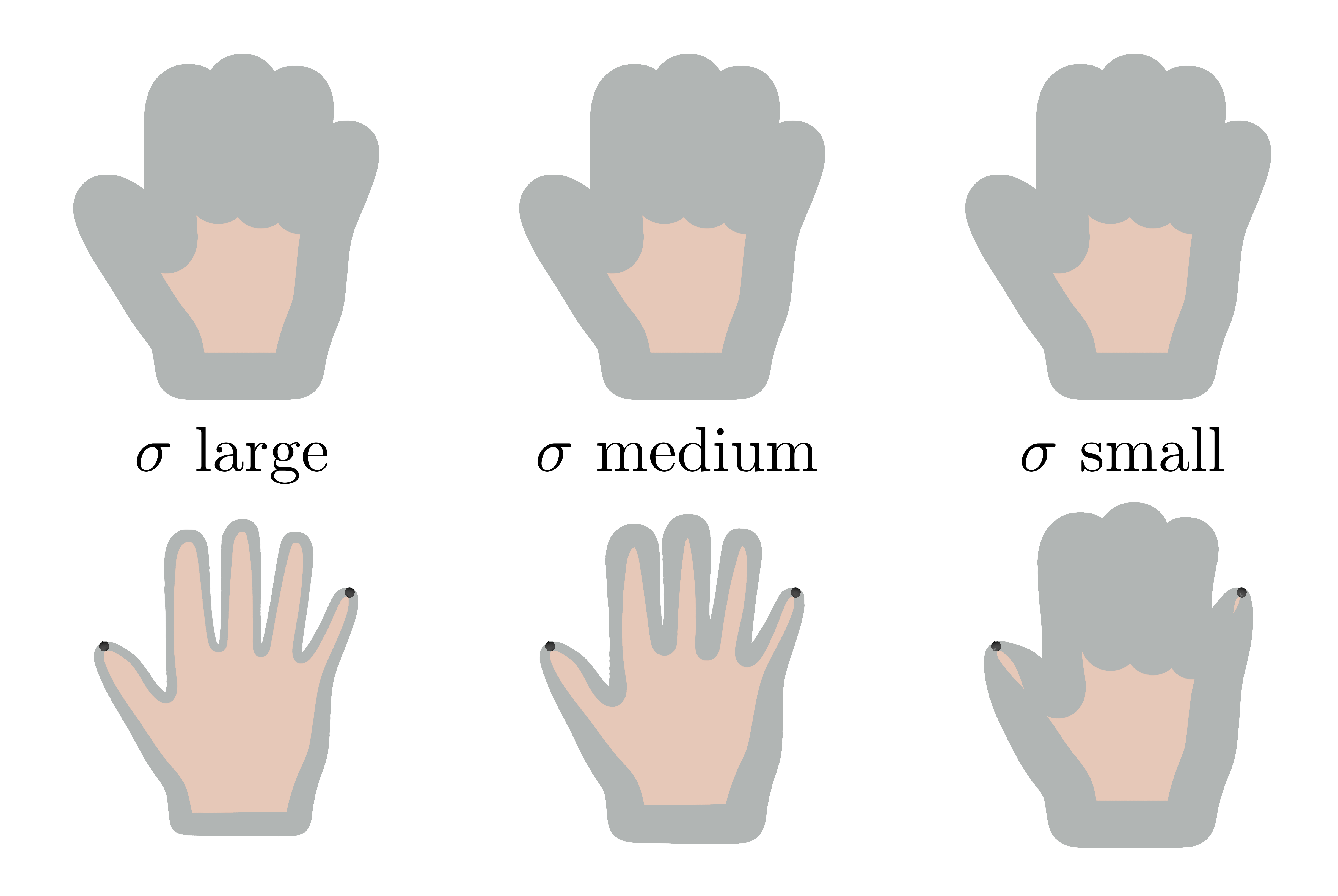
We start by discussing a Gaussian Process model of smooth deformations , where is the Gaussian kernel
We define models for three different values of . In the first model, we choose large compared to the size of the domain, in the second medium and in the third one a small value is chosen.
The top row in Figure 1 shows a confidence region (in grey) of the corresponding Gaussian Process models. As expected, the prior distribution is the same for all three models, irrespective of the choice of , as does not affect the size of the deformations but only their correlations. The bottom row in Figure 1 shows the posterior distributions given two observations (of the deformation) at the tip of the thumb and the little finger.
We notice for all the examples, that the variance at the point where the deformation is observed is small. Also, we can see that the larger is chosen, the stronger is the variance of the locations nearby this point affected by the observations. If is small, the effect is only very local. This is because the larger the value of is, the larger is the area where the deformations are influenced by the observations.
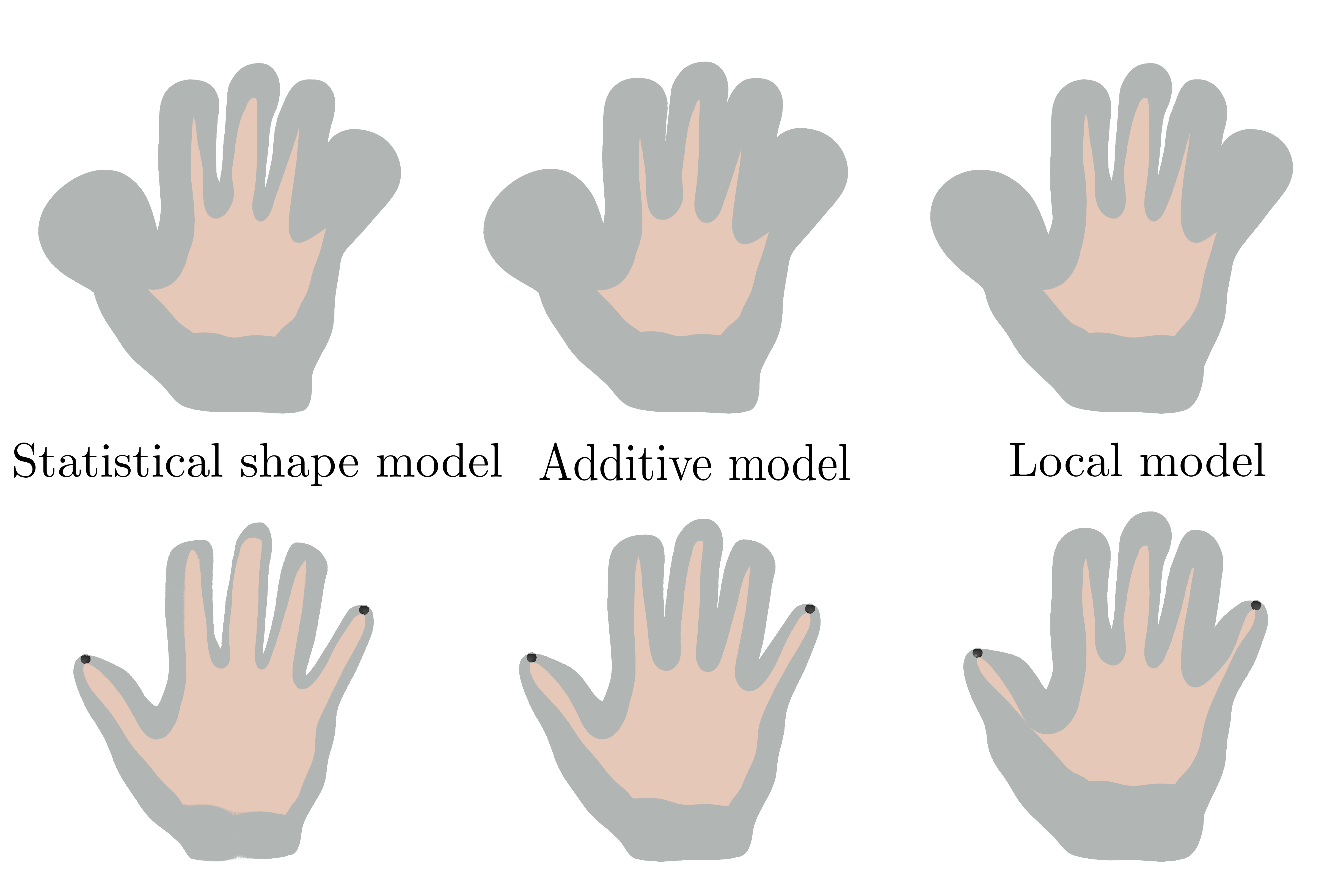
Statistical shape models learned from data
We explore now the same for the statistical shape models where the mean and covariance are estimated from data.
The top row in Figure 2 again shows the prior for three different models: the statistical model , an additive model where the flexibility is enlarged by modelling additional smooth deformation and a localised model where for details of these models). The confidence regions look almost the same for all prior models, only the additive model shows a slighly increased variance, which is expected as in this case two covariance functions are added. The posterior models are more interesting. We see that in the standard statistical shape model, the variance is reduced everywhere. This is why statistical models are often said to be global models - the knowledge about a single point influences the deformations of the full shape.
The situation is not much different for the additive model, except that there is slightly more variability left everywhere. The local model, however, shows considerably more variance in regions that are further away from the observed deformations, as the multiplication with the Gaussian kernel breaks the global correlations and hence the information about the known deformation does not influence the deformations in these regions.