The regression problem

A common task in shape modelling is to infer the full shape from a set of measurements of the shape. This task can be formalised as a regression problem. In the following, we quickly review the standard regression problem and discuss how it extends to shape modelling.

Standard regression problem​

Let $\{x_1, \ldots, x_n\} \subset \Omega$ be a fixed set of input points defined on some domain $\Omega$ and assume that there is an (unknown) function $f_0 : \Omega \to \mathbb{R}$, which generates values $y_i \in \mathbb{R}$ according to $y_i = f_0(x_i) + \epsilon_i, \, i = 1, \ldots, n.$ A common assumption is that $\epsilon_i$ is independent Gaussian noise, i.e. $\epsilon_i \sim N(0, \sigma^2)$. The function $f_0$ is called the regression function.

The regression problem is to infer the function $f_0$ from given observations $\{\tilde{y}_1, \ldots, \tilde{y}_n\}$ at the input points. Figure 1 (left) illustrates this setting. It is clear that, since we only have access to the function value at a finite number of points, there are in general many solutions that could have generated the data, as illustrated in Figure 1 (right).

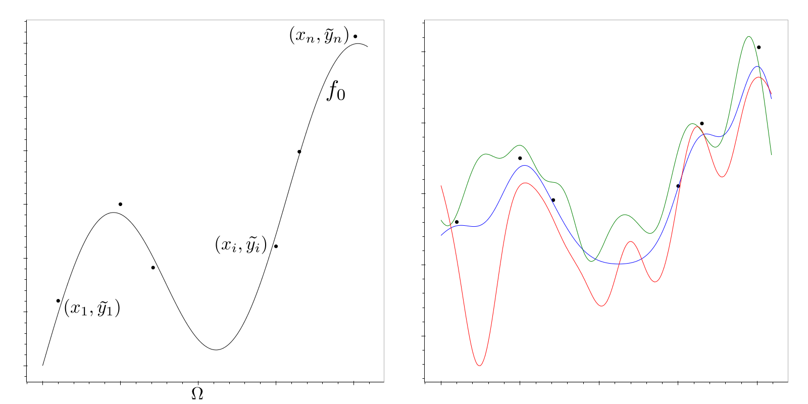
In order to obtain a well-posed problem with a unique solution, we need to make prior assumptions about the possible functions $f$ that could have generated the data. One possibility is to assume that the functions are distributed according to a Gaussian Process: $f \sim GP(\mu, k)$. In this case the problem is called Gaussian Process regression. Gaussian Process regression provides an elegant solution to the regression problem, and it turns out that this method has immediate applications in shape modelling. Before we explain this method in detail in the next video, we will quickly discuss how the regression setting extends to the case of shape modelling, and how the regression problem arises in shape modelling applications.

Regression in shape modelling​

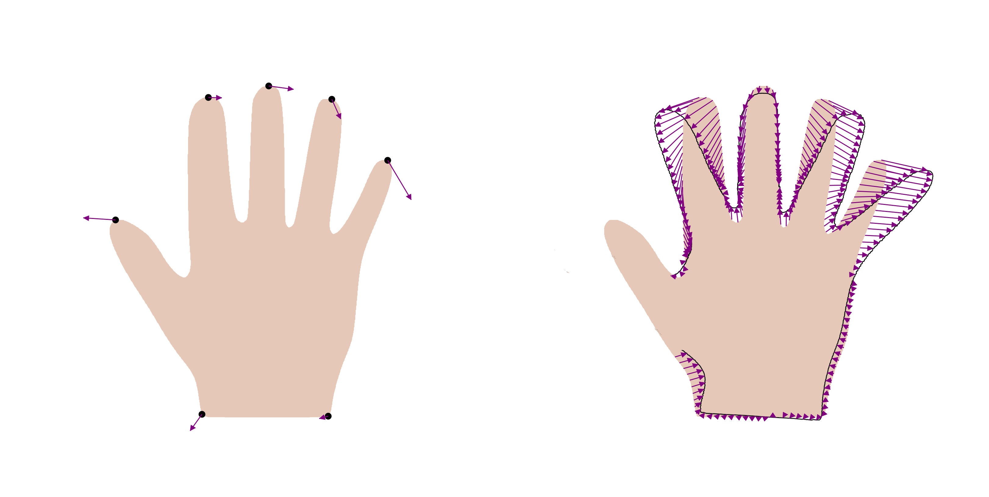
In shape modelling, the regression problem can be formulated as follows: the points $x_1, \ldots, x_n \subset \Gamma_R$ are points on the reference shape $\Gamma_R$. The regression model is defined as $u_i = u_0(x_i) + \epsilon$ where the regression function $u_0 : \Gamma_R \to \mathbb{R}^2$ is a deformation field and $\epsilon \sim N(0, \sigma^2 I_{2 \times 2})$ is independent Gaussian noise. Analogically to the standard setting, the goal is to infer the regression function $u_0$ from given observations $\{\tilde{u}_1, \ldots, \tilde{u}_n\}$. Figure 2 illustrates this setting.

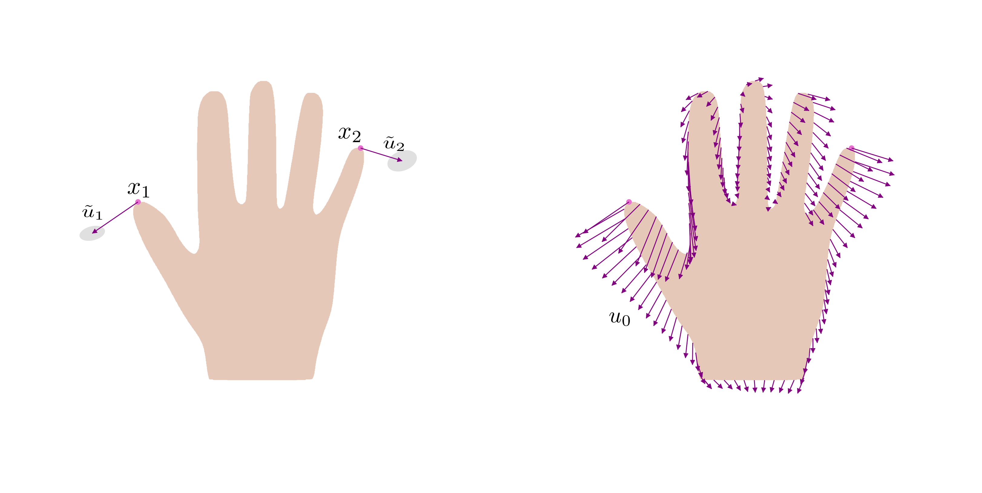
The possible deformations $u$ are modelled using a Gaussian Process model $GP(\mu, k)$ that models the shape variations of a given shape family.

There are two typical applications of the regression problem. The first one arises when we have obtained a sparse set of measurements of the shape and would like to infer the full shape (Figure 3, left). In the second application, it is possible to obtain an arbitrary number of measurements, but only for a part of the shape. This setting is typical for shape reconstruction problems, where we are given only a part of a shape and the goal is to infer the shape of the unseen part (Figure 3, right).