Enlarging the flexibility of statistical shape models

In the classical approach for building statistical shape models, all the shape variability that is represented by the model is learned from example data. This helps to ensure that all the shapes it represents are anatomically valid. However, there is also a disadvantage: the model can only represent shape variations that were observed in the example data.

For instance, if in a dataset of hand shapes the fingers are perfectly straight in all examples, the model will never be able to represent a crooked finger. If we have only little example data (which in practice is often the case), we cannot expect to observe the full shape variability. In this article, we will show how the rules for combining covariance functions can be used to overcome this limitation.

Limitations of classical statistical shape models​

We have seen that we can learn the shape variations from a set of example shapes that are in correspondence. Let $u_1, \ldots, u_n$ be the deformation fields that relate the reference shape $\Gamma_R$ with a set of observed example shapes $\Gamma_1, \ldots, \Gamma_n$. A statistical shape model is obtained by defining a Gaussian Process $GP(\mu, k)$, where the mean function $\mu$ is chosen to be the sample mean $\mu_s(x)= \frac{1}{n} \sum_{i=1}^n u_i(x), \, x \in \Gamma_R$ and the covariance function is the sample covariance $k_s(x,x') = \frac{1}{n} \sum_{i=1}^n (u_i(x) - \mu_s(x))(u_i(x') - \mu_s(x'))^T, \, x, x' \in \Gamma_R$ estimated from the data.

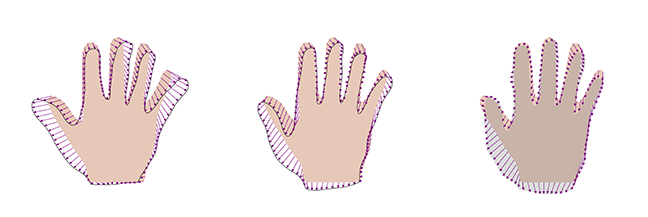
It turns out that the resulting Gaussian Process $GP(\mu_s, k_s)$ can only represent samples that are linear combinations of the example deformations $u_i, \, i = 1, \ldots, n$. In the extreme case, where we have only one sample, the resulting Gaussian Process will only represent multiples of the same example. This is illustrated in Figure 1.

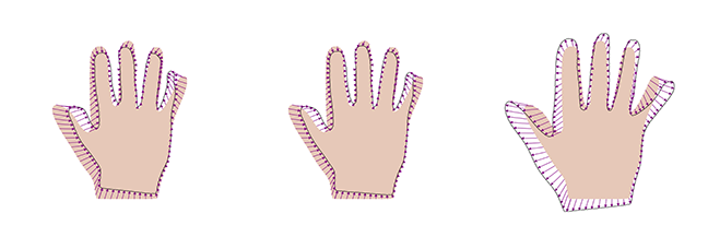
As a consequence, if we do not have a sufficient number of example shapes, the model will be unable to represent the full shape variations. This is illustrated in Figure 2, where we see the best representation of an anatomically valid hand shape (indicated by the grey area), when a model built from 4, 8 and 12 datasets is used. We see that the approximation is getting better the more examples we add, but even with 12 examples, we cannot represent the shape accurately.

It turns out that the methods for combining covariance functions we discussed before lead to elegant solutions for working around this problem.

Modelling the missing variability​

We see in Figure 2 that the part of the shape that the model cannot explain corresponds to a smoothly varying region. The simple idea is that if the model could represent general smooth deformations, the missing part could be explained too by the model. Smooth deformation fields can be modelled well using a Gaussian kernel. By adding the kernels together, we can augment the learned shape deformations with the more general model of smooth deformations. This results in the new model $GP(\mu_s, k_s(x,x') + s I_{2 \times 2} \exp(-\frac{||x-x'||^2}{\sigma^2})).$

Here we choose the parameter s such that it coincides approximately with the average error that we see (since this is the added variance in the resulting covariance function) and $\sigma^2$ is chosen relatively large, to reflect the fact that the error is highly correlated.

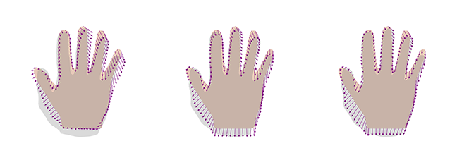
It is important to validate the shape deformations generated by the model by visual inspection. Figure 3 shows two samples obtained from this model as well as the best representation of the target hand using this new model. We see that the samples still look reasonable. Furthermore, we get a perfect representation of the target shape, even though we used only 8 examples, which had led to a large error before.

Localised shape models​

We can also enlarge the shape variability of the learned model by multiplying the kernel $k_s$ with a Gaussian kernel, i.e. by defining the model $GP(\mu_s, k_\text{local}),$ with $k_\text{local}(x,x’)=k_s(x,x') \odot I_{2 \times 2}\exp(-\frac{||x-x'||^2}{\sigma^2})$.

The intuition is the following: if we have 8 datasets to model the full hand, these might not be sufficient to represent all shape variations, as there are many complex variations and hand configurations possible that the model needs to account for. However, if we were to use the same 8 datasets to explain only, say, the thumb, 8 examples could be sufficient. The same holds for any other part of the shape. This is exactly what the multiplication achieves. We see that for any point $x$, the covariance $k_\text{local}(x,x')$ with any other point $x'$ is virtually 0 if $\newcommand{\norm}[1]{\left\lVert#1\right\rVert} \norm{x-x'}$ is large. Hence, the new kernel has the effect of suppressing global correlations, but preserves the learned correlations locally.

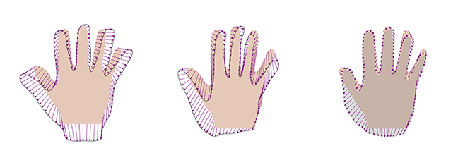
Figure 4 shows samples and the best representation for this case. We see that, in this case also, the samples still look like valid hand shapes, while this approach can also perfectly represent the target hand.