Sampling from a shape model
We have seen that, thanks to the marginalisation property of a Gaussian Process, any finite marginal distribution is a multivariate normal distribution. One important consequence of this is that we can sample from the model to generate new shapes from the shape family.
Sampling from a probability distribution is the task of generating concrete values (samples) of a random variable, according to the probabilities defined by the distribution. With this process, samples of high probability are more likely to be generated than those with a low probability. Note that this use of the term sampling should not be confused with the process of sampling a continuous function, where the goal is to obtain a discrete representation of the function.
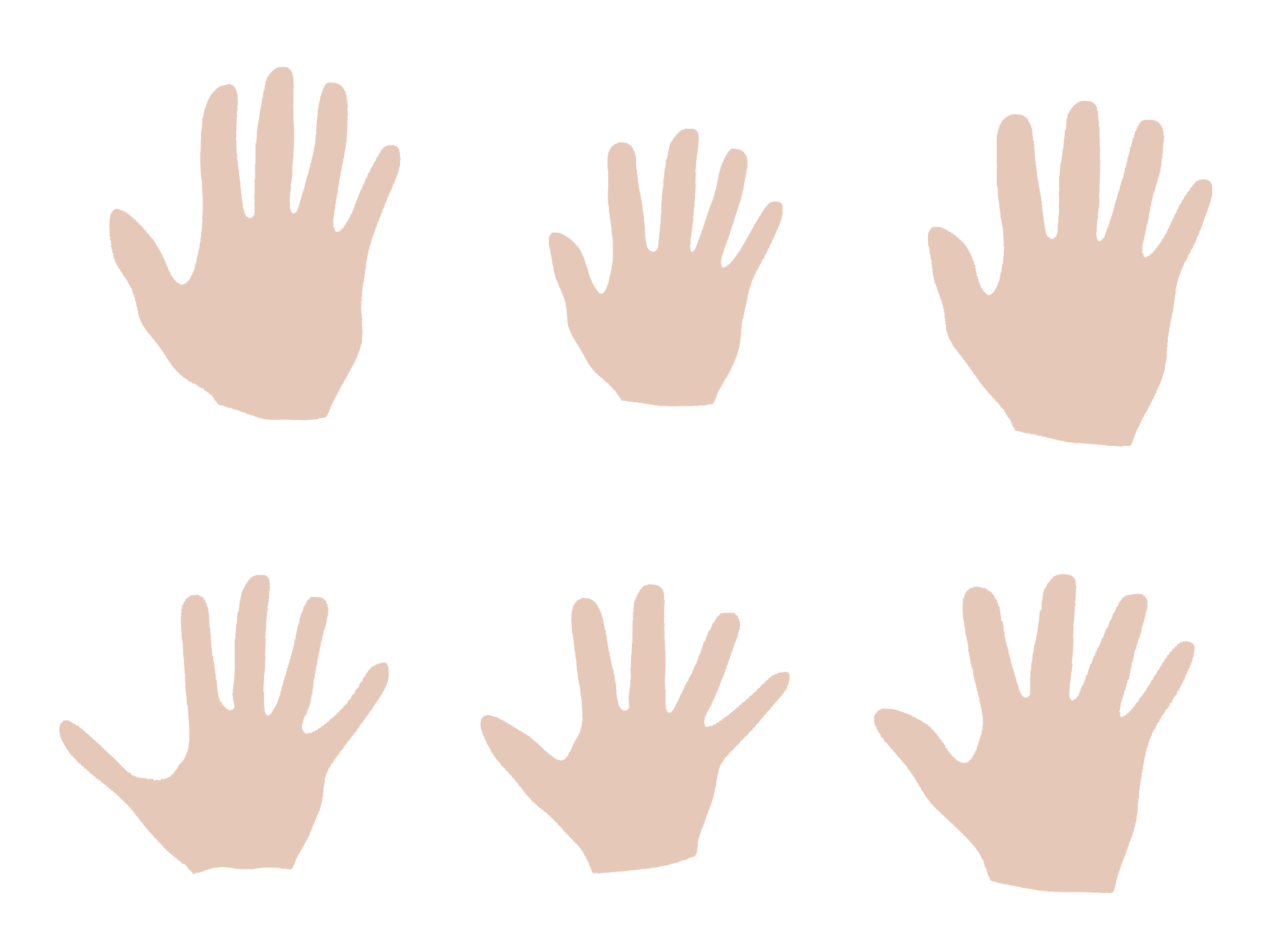
In our application, the values of the random variable are deformation fields, which represent shape variations. The possibility to sample these deformation fields thus gives us a means to generate new shapes. Figure 1 shows a number of samples from our hand model. Looking at the sampled hand shapes, we get a visual impression of the variability of this shape family. For instance we can see immediately that the main sources of shape variability are the size of the hands and how much the fingers are spread.
Sampling shapes is maybe the simplest possible use of shape models. Nevertheless it has many practical applications. For a medical student, sampling shapes might be a useful way to learn about the shape variations of an anatomical structure. For a designer of medical implants, samples can be used for generating representative data for a shape family, in order to test whether an implant design fits the typical shapes that occur in a population. For us as developers of a model, sampling is an invaluable diagnostic tool to check if the model that we computed is reasonable.
Sampling from a multivariate normal distribution
Unlike for many other distributions, sampling from a multivariate normal distribution is straight-forward. The general procedure is as follows:
Let be a multivariate normal distribution with mean and covariance matrix .
- Generate random numbers where by calling multiple times a scalar Gaussian random number generator (which is readily available in most programming languages). Define the vector .
- Compute using the Cholesky decomposition. Here is a lower triangular matrix, which results from this decomposition.
- Compute the sample , which has the desired distribution.
A downside of this procedure is, however, that we need to have access to the full covariance matrix . In practical shape modelling applications, this matrix is often too large to be stored explicitly. As we will see later this week, there are ways to sample from a shape model that do not suffer from this problem and even allow us to explore the variability in a systematic way.