How does this course work

Course structure​

Every week starts with a theory part that introduces the concepts and mathematical methods behind shape modelling. The theory part is complemented by a practical block, in which you will learn how to apply the theoretical concepts using the software Scalismo. This will enable you to visualise and explore the mathematical concepts by yourself, which we believe is a very effective way to understand and digest the theory.

Besides the theoretical concepts you will also learn the basic data structures and concepts of the Scalismo software. At the end of the course you will be able to use all the concepts that we explain in this course in your own shape modelling applications. This track is the prerequisite for being able to participate in the shape modelling project that starts in Week 4 of the course. If you want to follow this track, some programming experience using a modern language (such as e.g. Python, Java or C++) is recommended.

Course overview​

During your learning journey you will reach several different milestones:

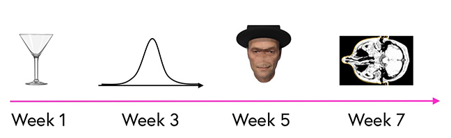
Week 1 of the course gives you a very general introduction in the topic of shape modelling, and introduces the software. After this week you will have sufficient information that you can survive at a cocktail party when people talk about shape modelling. You will also have the software environment ready and will have done your first simple steps with Scalismo.

In Weeks 2 to 4 we will discuss the mathematical concepts behind shape models and how you can learn shape variations from example data. After Week 3 you will be able to understand classical statistical shape models, the modelling assumptions that are made and how you can use shape models for studying shape variations. In Week 4, we will also show you how these concepts can be generalized to a much broader class of shape models defined by a Gaussian Process.

In Week 5 we will discuss how missing parts of a shape can be predicted using a shape model. After this week, you will be able to complete the first milestone, namely to compute a suitable nose for a face.

In Weeks 6 and 7 we will discuss how surfaces and images can be analysed using shape models and derive a simple fitting algorithm. We will also show you how the same fitting algorithm, used with the general Gaussian Process models introduced in Week 4, will give rise to a powerful method for registration, which is the last tool needed to complete the shape modelling toolchain.

In Week 8 we wrap up the course and give a brief outlook on how shape models are used in computer vision to analyse 2D photographs of faces.

Gaussian Processes​

The theoretical core concept around which this course is built is that of a Gaussian Process. Traditionally, there has been a distinction between shape models that are learned from example data (called statistical shape models or point distribution models) and analytical models, such as for example spline models. Gaussian Processes unify both types of models and make it even possible to freely combine them. As we will see towards the end of the course, this allows us to understand all the tools we need in a typical shape modelling application using a single mathematical concept. This does not only make it easier to understand shape modelling, but also greatly simplifies the algorithms and tools used in practical shape modelling applications.

Glossary​

In case you are unclear about some technical terms introduced in the course, please make sure to check our Glossary.